NEWSnews
Relay Protection Test Set: Overcurrent Test, Six Tests & Setting Calculations
Chapter 4 Worked Example: How to Perform an Overcurrent Protection Test
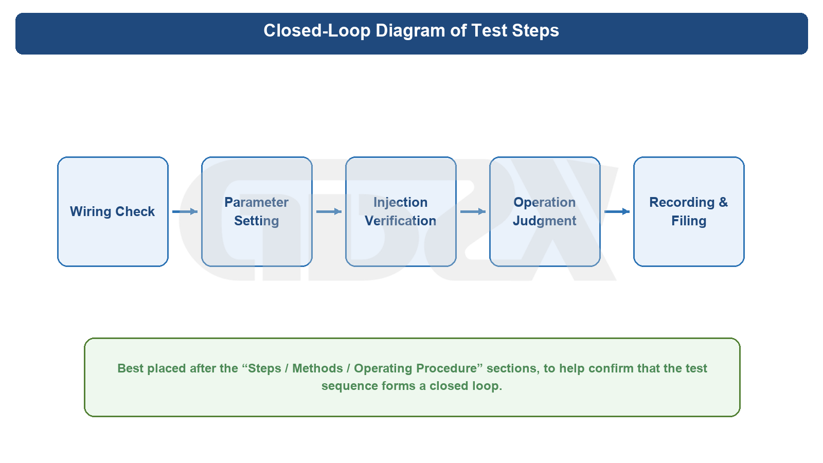
Diagram: Closed-Loop Diagram of Test Steps
This section presents the most common, most hands-on engineering example: the operating-value and operating-time test of a 10 kV line overcurrent protection. Software interfaces of test sets from different manufacturers vary, but the core approach is basically the same.
4.1 Test Scenario Setup
Assume that the overcurrent Stage II settings of a feeder protection device are as follows:
• Overcurrent Stage II setting current: 600 A (primary value)
• Overcurrent Stage II operating time: 0.50 s
• CT ratio: 600/5
Conversion by the CT ratio:
600/5 means that a primary current of 600 A corresponds to 5 A on the secondary side
Therefore, the 600 A setting converted to the secondary side equals 5.0 A
That is, the target values for the test set to focus on in this test are:
• Reference operating current: 5.0 A
• Reference operating time: 0.50 s
4.2 Pre-Test Preparation
1. Confirm that the work permit, safety measures, and device status satisfy the test conditions.
2. At the CT terminal side, complete short-circuiting first and disconnecting afterwards as required by the regulations, isolating the current input of the protection under test from the in-service circuit.
3. Check that the settings in the protection device are consistent with the test sheet, and confirm that this test targets Overcurrent Stage II.
4. Clarify whether this test uses single-phase injection or three-phase injection; if only the operating value of one overcurrent stage is to be verified, single-phase injection is usually sufficient.
5. Confirm that the digital input channels of the test set are intact, so as to acquire the protection trip output signal.
4.3 How to Wire for This Test
Taking the Phase A overcurrent test as an example, the most common wiring approach is as follows:
1. Connect the test set IA current output terminal to the IA current input terminal of the protection device.
2. Connect the test set current common terminal IN to the corresponding current common terminal of the protection device.
3. Connect both ends of test set digital input DI1 to both ends of the protection device trip output contact.
4. If only the overcurrent protection test is performed this time, the voltage terminals may be left unconnected.
This can be understood with the simplified diagram below:
Test set current output Protection device
IA -------------------------> IA
IN -------------------------> IN (current common terminal)
Test set digital input Protection device output contact
DI1+ ------------------------> one end of the trip output
DI1- ------------------------> the other end of the trip output
If the on-site device uses three-phase four-wire or separate-phase independent terminals, the terminal names may be Ia, Ib, Ic, In, or manufacturer designations such as A411, A421, but the wiring principle remains unchanged: current output to current input, digital input acquisition to the output contact; isolate the in-service circuit before injection.
Emphasizing the operating sequence once again:
• First short-circuit the secondary circuit at the CT terminal block side
• Then disconnect the original current input wiring of the protection device
• Then connect the test set to the input terminals of the protection device
• After the test is completed, first restore the original circuit, then remove the short-circuiting links
4.4 Step-by-Step Operating Procedure
Step 1: First perform the “no-operation” check
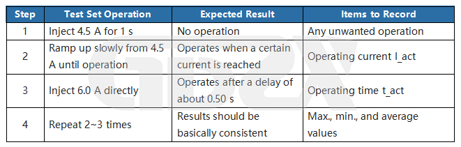
Set the test set output to 0.9 × 5.0 A = 4.5 A, and apply a stable current for a duration longer than the set time, e.g. 1 s.
Expected results:
• The protection device should not operate
• The test set should not acquire a trip output
The purpose of this step is to first verify that the protection will not “maloperate” because its actual operating value is lower than the setting.
Step 2: Measure the operating current
Keeping the time setting unchanged, raise the injected current step by step in a slow ramp, for example:
• Start from 4.5 A
• Increase by 0.1 A
• Hold each step for 1~2 s
When the protection operates, record the output current value I_act at the moment of operation.
Example:
• If the measured operation occurs at 5.1 A, the operating error is
Operating error (%) = |5.1 - 5.0| ÷ 5.0 × 100% = 2%
If the device technical specification requires the operating value error not to exceed ±3%, this item is judged as qualified.
Step 3: Measure the operating time
Raise the test set output directly to 1.2 × 5.0 A = 6.0 A, start timing at the instant the current is applied, and stop timing at the instant the protection trip output is acquired, obtaining the operating time t_act.
Example:
• Setting time: 0.50 s
• Measured time: 0.52 s
Then the time error is:
Absolute time error = |0.52 - 0.50| = 0.02 s = 20 ms
Relative time error (%) = |0.52 - 0.50| ÷ 0.50 × 100% = 4%
Whether this is qualified should be judged according to the device technical specification and current regulations; for many common scenarios, a deviation of 20 ms is usually acceptable, but the actual acceptance criteria prevail.
Step 4: Repeatability verification
Repeat the measurement of the same item at least 2~3 times, and observe whether the operating current and operating time show excessive dispersion.
If any of the following occurs, pause and investigate:
• Under the same injection conditions, operation is intermittent
• The operating time fluctuates greatly
• The operating value deviates significantly from the setting
4.5 The Whole Process in One Flow Table
4.6 The Three Most Common Field Problems
Problem 1: Can I just apply a large current right away? You can do the time test this way, but it is not advisable to skip the “no-operation check” and the operating value verification; otherwise it is difficult to detect setting deviations or unwanted operation.
Problem 2: The operating time is too long — is the protection broken? Not necessarily. First confirm whether the digital input is connected to the protection output rather than to the circuit breaker auxiliary contacts; otherwise the breaker mechanical time will be included in the measurement.
Problem 3: It never operates — what to check first? Check three things first: whether the setting value is entered correctly; whether the primary value is correctly converted to the secondary value; whether the wiring and phase correspondence are correct.
4.7 The Value of This Example
If the reader is encountering relay protection test sets for the first time, truly understanding this example means mastering the most fundamental main line:
Obtain the settings → convert to secondary values → wire correctly → perform the no-operation check first → then verify the operating value and operating time → finally judge against the standard and record.
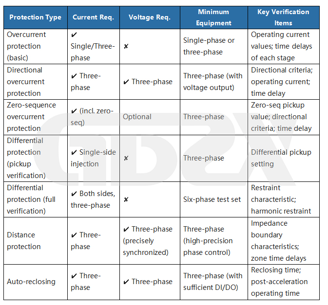
Chapter 5 In-Depth Analysis of Six Typical Tests
Chapter 6 Setting Calculation Formulas and Test Verification Methods
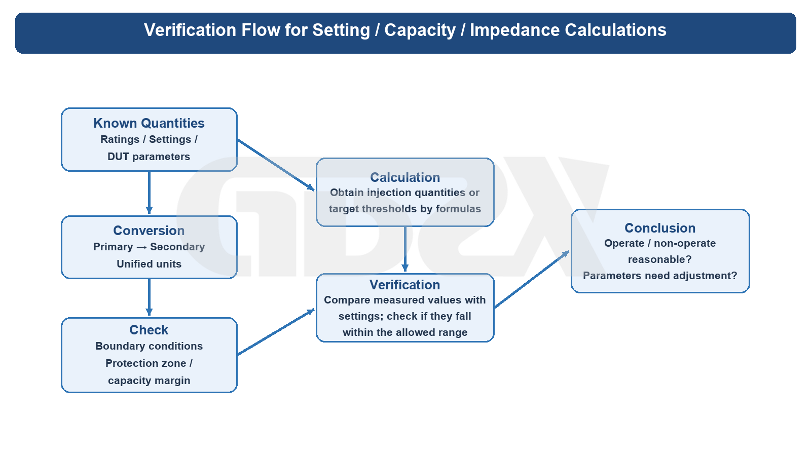
Diagram: Verification Flow for Setting / Capacity / Impedance Calculations
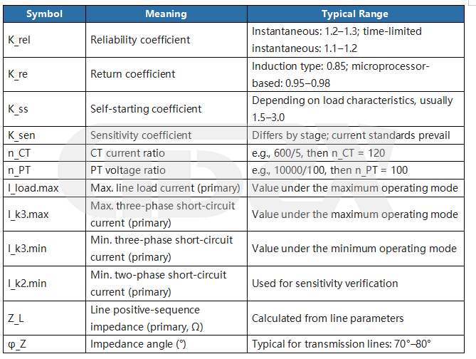
This chapter is the core technical chapter; all formulas are expressed with common engineering plain-text symbols, and a unified symbol table is attached below.
Master Symbol Table
5.1 CT Ratio Conversion (the Prerequisite of All Tests)
Before any setting value is entered into the test set, it must first be converted from the primary value to the CT secondary value.
I_set(secondary) = I_set(primary) ÷ n_CT
Example:
• Overcurrent Stage II primary setting = 600 A
• CT ratio = 600/5, i.e., n_CT = 120
• Secondary current to be injected by the test set = 600 ÷ 120 = 5.0 A
5.2 Overcurrent Protection Setting Calculation
5.2.1 Overcurrent Stage I (instantaneous protection)
Set to ride through the maximum three-phase short-circuit current at the end of this line:
I_set.I(primary) = K_rel × I_k3.max(line end)
Secondary value:
I_set.I(secondary) = I_set.I(primary) ÷ n_CT
5.2.2 Overcurrent Stage II (time-limited instantaneous)
Set to ride through the maximum three-phase short-circuit current at the end of the next line section:
I_set.II(primary) = K_rel × I_k3.max(next-section end)
Secondary value:
I_set.II(secondary) = I_set.II(primary) ÷ n_CT
5.2.3 Overcurrent Stage III (overload protection)
Set to ride through the maximum load current:
I_set.III(primary) = (K_rel × I_load.max) ÷ (K_re × K_ss)
Secondary value:
I_set.III(secondary) = I_set.III(primary) ÷ n_CT
5.2.4 Sensitivity Verification
The sensitivity coefficient of each protection stage must be verified and must meet the regulation requirements (current valid standards prevail):
K_sen = I_k2.min(protection zone end, primary) ÷ I_set(primary)
Where I_k2.min is the minimum two-phase short-circuit current at the end of the protection zone (under the minimum operating mode).
5.3 Verification Methods for Overcurrent Protection Tests
5.3.1 Operating Current Verification
1. Set the test set output current to 0.9 × I_set(secondary); the protection should not operate;
2. Increase the current slowly, and record the output current I_act at the moment the protection device operates;
3. Calculate the operating error:
Operating error (%) = |I_act - I_set(secondary)| ÷ I_set(secondary) × 100%
Reference acceptance criterion (typical value, subject to the device technical specification): operating error ≤ 3%
5.3.2 Operating Time Verification
The test set applies a stable current of 1.2 × I_set(secondary), measures the protection operating time t_act, and calculates the error:
Absolute time error = |t_act - t_set|
Relative time error (%) = |t_act - t_set| ÷ t_set × 100%
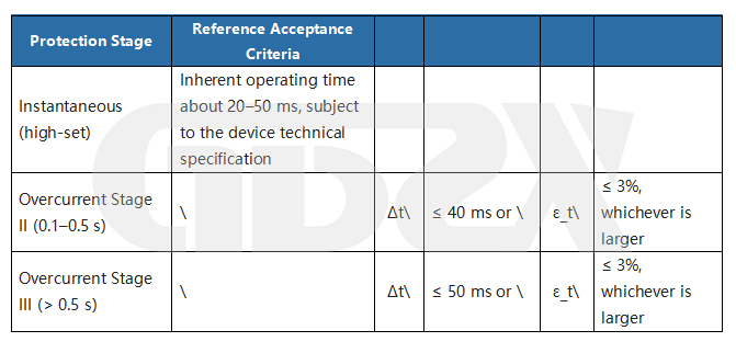
Reference acceptance criteria (typical values, subject to the device technical specification):
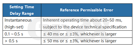
The above are reference ranges; the actual acceptance criteria are subject to current valid standards and the device technical specification.
5.4 Zero-Sequence Overcurrent Protection Calculation
5.4.1 Composition of the Zero-Sequence Current
During normal balanced three-phase operation, the zero-sequence current is approximately zero; when a single-phase-to-ground fault occurs, the sum of the three phase currents becomes significantly non-zero:
3I0 = Ia + Ib + Ic
Normal operation: 3I0 ≈ 0
Single-phase-to-ground fault: 3I0 increases significantly (fault characteristic)
5.4.2 Zero-Sequence Protection Setting
I_0set(secondary) = (K_rel × I_0.unbalance.max) ÷ n_CT(zero-seq CT)
Where I_0.unbalance.max is the maximum permissible unbalanced zero-sequence current during normal operation.
5.4.3 Two Methods for the Test Set to Simulate the Zero-Sequence Current
Method 1: Unbalanced three-phase injection
Inject the fault current Ia into phase A only, with the phase B and C currents set to zero; the equivalent zero-sequence component is:
I0 = (Ia + 0 + 0) ÷ 3 = Ia ÷ 3
i.e., 3I0 = Ia
Therefore, when the test set injects Ia = I_0set(secondary), the zero-sequence current measured by the protection equals I_0set.
Method 2: Dedicated zero-sequence output port
Some test sets provide a dedicated zero-sequence current output port that can directly output 3I0 to the zero-sequence CT input of the protection device, with no conversion required.
5.5 Distance (Impedance) Protection Calculation
5.5.1 Measured Impedance of the Protection Device (for ground faults)
The protection device calculates the apparent impedance from its installation point to the fault point:
Z_app = U_ph ÷ (I_ph + K0 × 3I0)
Where the zero-sequence compensation factor K0 is determined by the line parameters:
K0 = (Z_L0 - Z_L1) ÷ (3 × Z_L1)
Z_L1 is the positive-sequence line impedance, and Z_L0 is the zero-sequence line impedance.
For a three-phase short circuit (no zero-sequence component, 3I0 = 0), the formula simplifies to:
Z_app = U_ph ÷ I_ph
5.5.2 Zone Setting Impedances (primary values)
Zone I: Z_set.I(primary) = K_rel × n_I × Z_L (n_I usually 0.80–0.85)
Zone II: Z_set.II(primary) = K_rel × (Z_L + n_II × Z_L.next) (n_II usually 0.70–0.80)
5.5.3 Converting Primary Impedance to Secondary Impedance (test set input value)
Z_set(secondary) = Z_set(primary) × n_CT ÷ n_PT
5.5.4 Calculating the Test Set Injection Quantities
To simulate a fault point with an impedance of Z_sim, the injected current and voltage must satisfy:
U_output = I_output × Z_sim
The angle by which the voltage leads the current (impedance angle):
φ_Z = arctan(X_sim ÷ R_sim)
Where Z_sim = R_sim + jX_sim (the resistive and inductive components of Z_sim).
Typical impedance angle range for transmission lines: 70°–80°.
5.5.5 Complete Numerical Example
Given conditions:
Positive-sequence line impedance (primary): Z_L = 10 Ω, impedance angle φ_Z = 75°
CT ratio: n_CT = 200/5 = 40
PT ratio: n_PT = 110000/100 = 1100
Zone I setting ratio: n_I = 0.80, reliability coefficient K_rel = 0.85
Step 1: Calculate the primary Zone I setting impedance
Z_set.I(primary) = K_rel × n_I × Z_L
= 0.85 × 0.80 × 10
= 6.80 Ω
Step 2: Convert to the secondary impedance
Z_set.I(secondary) = Z_set.I(primary) × n_CT ÷ n_PT
= 6.80 × 40 ÷ 1100
= 272 ÷ 1100
≈ 0.247 Ω
Step 3: Test set settings
Injected current: I = 5.00 A (rated current)
Corresponding injected voltage: U = I × Z_set.I(secondary) = 5.00 × 0.247 = 1.24 V
Angle by which the voltage leads the current: φ = 75°
Step 4: Verification judgment
Simulated impedance < 0.247 Ω (i.e., lower U) → measured impedance falls inside Zone I → protection should operate
Simulated impedance > 0.247 Ω (i.e., higher U) → measured impedance outside Zone I → protection should not operate
By measuring point by point around 0.247 Ω, the actual Zone I operating boundary can be determined and compared with the setting.
5.6 Differential Protection Calculation
5.6.1 Definitions of Differential and Restraint Currents
For a double-ended differential protection (taking transformer differential protection as an example), after phase compensation and balancing-coefficient correction of the currents on both sides:
Id = |I1’ + I2’| (differential current, fault characteristic)
Ir = (|I1’| + |I2’|) ÷ 2 (restraint current, larger for external faults)
I1’ and I2’ are the per-side converted currents after phase compensation and magnitude balancing.
5.6.2 Percentage Differential Restraint Characteristic (multi-slope characteristic)
Operating conditions of the differential protection (typical three-section broken-line characteristic; specific parameters are subject to the device settings):
① Pickup section (Ir < Ir.break1):
Operating condition: Id ≥ Id.min
Id.min is the differential pickup setting (setting parameter)
② Percentage restraint section (Ir.break1 ≤ Ir < Ir.break2):
Operating condition: Id ≥ K1 × Ir
K1 is the low restraint coefficient (setting parameter, typically 0.3–0.5)
③ High restraint section (Ir ≥ Ir.break2):
Operating condition: Id ≥ K2 × Ir
K2 is the high restraint coefficient (setting parameter, K2 > K1)
Ir.break1 and Ir.break2 are the break-point restraint currents of the characteristic (setting parameters).
Verification method: select several operating points near the characteristic curve in the (Ir, Id) plane, measure point by point whether the protection operates, plot the measured boundary, and compare it with the set characteristic curve.
5.6.3 Transformer Balancing Coefficient Calculation
The CT current magnitudes on different sides of a transformer differ, so balancing coefficients are applied to make the differential current zero under normal operation. Taking a two-winding transformer with the high-voltage side as the reference:
HV-side balancing coefficient K_bal.H = 1 (reference side)
LV-side balancing coefficient K_bal.L = I_N.H ÷ I_N.L
= (S_N ÷ (√3 × U_N.H)) ÷ (S_N ÷ (√3 × U_N.L))
= U_N.L ÷ U_N.H
S_N is the transformer rated capacity; U_N.H and U_N.L are the rated voltages of the HV and LV sides.
Microprocessor-based protection devices usually complete the compensation automatically, but during testing the test set must correctly input the transformer rated voltages and vector group (e.g., Yd11) to construct the test currents correctly; otherwise, even with correct protection logic, the test results will deviate.
5.6.4 Harmonic Restraint Criterion (Inrush Identification)
Energizing a transformer at no load produces a magnetizing inrush current rich in second-harmonic content (100 Hz). Differential protection uses harmonic restraint to prevent unwanted operation during inrush:
Criterion: I_2nd ÷ I_1st ≥ K_2H → identified as inrush → block the differential protection
K_2H is the harmonic restraint ratio setting (typically about 15%–20%, subject to the device settings)
Composite waveform output by the test set:
i(t) = I_1st × sin(ωt + φ1) + I_2nd × sin(2ωt + φ2)
ω = 2π × 50 = 314 rad/s (fundamental angular frequency)
2ω = 628 rad/s (second-harmonic angular frequency, 100 Hz)
Verification steps:
Step 1: Set I_2nd ÷ I_1st > K_2H (e.g., 20%)
→ the protection should identify it as inrush, block the differential, and not operate ✓
Step 2: Set I_2nd ÷ I_1st < K_2H (e.g., 10%)
→ the protection should identify it as an internal fault, and the differential should operate ✓
5.7 Operating Time Measurement Error Calculation
Absolute time error: Δt = t_act - t_set
Relative time error: ε_t(%) = Δt ÷ t_set × 100%
Where t_act is the operating time measured by the test set, and t_set is the set time delay of the protection device.
Reference acceptance ranges for the operating time of each protection stage (subject to the device technical specification):